
Mountain Birdwatch Overview (2010 to present)
Mountain Birdwatch monitors the breeding bird community of high-elevation spruce-fir forests in the northeastern United States, including Maine, New Hampshire, Vermont, and the Catskill and Adirondack Mountains of New York. These forests support a unique assemblage of boreal bird species that reach the southern limit of their breeding ranges in this region.
To establish the monitoring network in 2010, we used a model of Bicknell’s Thrush breeding habitat (Lambert et al. 2005) as a proxy for the distribution of spruce-fir forests across the Northeast. Sampling routes were selected using generalized random tessellation stratified sampling (GRTS) to provide spatially balanced coverage of these high-elevation habitats.
Each Mountain Birdwatch route contains 3–6 fixed sampling stations located along hiking trails or old logging roads. Stations occur between 573 and 1500 meters in elevation (mean ≈ 1009 m), with most located within the spruce-fir zone or the hardwood–boreal transition.
Since 2010, hundreds of volunteer community scientists have contributed surveys across nearly 800 long-term sampling stations, creating the most comprehensive monitoring datasets for high-elevation birds in the northeastern United States.
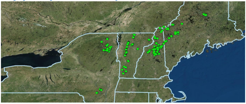
All ~800 Mountain Birdwatch sampling stations.
Survey Protocol
Mountain Birdwatch surveys focus on 10 focal bird species and one mammal species (Red Squirrel), which is an important nest predator of montane birds. However, the vast majority of Mountain Birdwatch observers record counts of all avian species.
Each survey consists of four consecutive 5-minute point counts conducted at a sampling station, for a total observation period of 20 minutes per station. Observers record the number of individuals detected during each 5-minute interval and indicate whether detections occur within or beyond 50 meters of the station.
The repeated-count format is a key strength of the Mountain Birdwatch protocol because it allows statistical models to account for birds that are present but not detected by observers.
Surveys are conducted during June, the period of peak breeding activity for the focal species. Counts begin 45 minutes before local sunrise and are typically completed before 8:00 AM. Surveys are conducted only under fair weather conditions (no rain and light wind), as poor weather can reduce detectability. The vast majority of detections are made by sound because the dense forest structure limits visual observations.
Data Analysis
Mountain Birdwatch data are analyzed using hierarchical community N-mixture models implemented in R and JAGS. These models estimate population abundance while accounting for imperfect detection by observers.
The models use the repeated counts at each sampling station to estimate detection probability separately from abundance. This allows population trends to be estimated even when some birds present at a station are not detected during surveys.
Abundance is modeled as a species-specific function of:
- long-term population trends over time
- geographic region
- elevation
- latitude
Detection probability is modeled using survey conditions that can influence detectability, and pooled across species, including:
- start time relative to sunrise
- wind conditions
- date within the breeding season
The community modeling framework allows information to be shared across species while still estimating species-specific trends. Model outputs are used to estimate both annual population trends and cumulative population change across the monitoring period.